Mapping your 2017 Geolocations: The Tidy Way

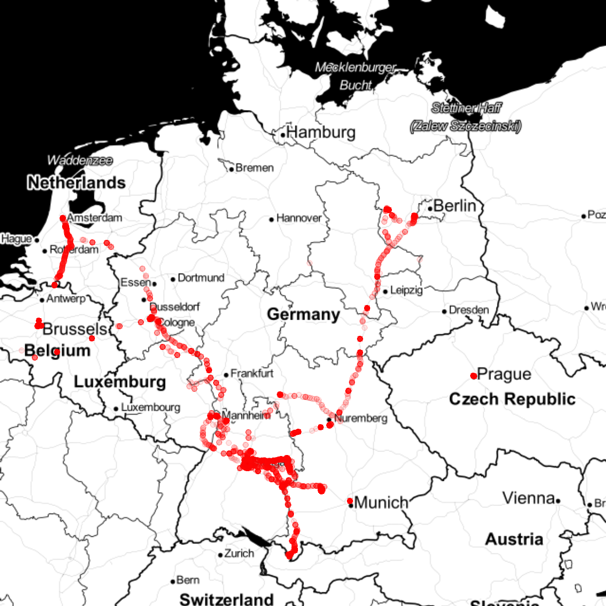
A few days ago I stumbled upon an instagram user who created a cool map of his geolocations. You can get his code here. I had to reproduce these cool maps myself and why not also make a blogpost while doing so?

The code for this blogpost can be found in this GitHub Repository.

Getting Started

First I need my geolocation data. If you use Google and own an Android cell phone, you can download yours here.

Now in Rstudio, I load in the needed packages:

pacman::p_load(ggmap, jsonlite, tidyverse, lubridate, magrittr)

After I put the downloaded .json file into my working directory, I use fromJSON to read in the data.¹

loc_history <- fromJSON('data/Standortverlauf.json')

As a next step, we want to extract our locations from the data. The locations are located (ha!) under loc_history$locations.

locations <- loc_history$locations #we are only interested in locations

Now comes the data wrangling part. We want the data to be in the right format. Especially the dates are easily transformed with the powerful lubridate package. First we create a time variable, using the as_datetime function. Next we bring the longitudes and lattitudes in the right format, then we select three relevant variables time, lon and lat. Lastly, we filter the dataframe so that we will only be left with data of 2017.

locations %<>% 
 mutate(time = as_datetime(as.numeric(timestampMs) / 1000)) %>% 
 mutate(lon = longitudeE7/1E7) %>% 
 mutate(lat = latitudeE7/1E7) %>% 
 select(time, lon, lat) %>% 
 filter(time > as_datetime("2017-01-01 00:00:01") & time < as_datetime("2017-12-31 23:59:59"))

Finally, we come to the plotting part! We type in our keyword and off we go with the ggmap package!

map1 <- "Stuttgart" %>% 
  qmap(maptype = "toner", source = "stamen", zoom = 14) + # creates the map
  geom_point(aes(x = lon, y = lat),                       # adding your data
             size = 1,
             data = locations,
             color = "red", 
             alpha = 0.01)
map1

We could also zoom out and get a map from all of Germany

map2 <- "germany" %>% 
  qmap(maptype = "toner", source = "stamen", zoom = 5) + # creates the map
  geom_point(aes(x = lon, y = lat),                       # adding your data
             size = 1,
             data = locations,
             color = "red", 
             alpha = 0.01)
map2

If we wanted to save the map on our computer, we could use the following code:

ggsave(map2, file = "images/map2.png", height = 4, width = 4)