For anyone who is interested in exploring the Democratic primary debates of the U.S. Presidential Election, I compiled a dataset with all debates so far (i.e.: 8).
In the following blog post I will introduce the R package
demdebates2020 which will be updated to include data from all
Democratic debates as they are held. Further, I will present some
possible use-cases and an exploratory analysis of the debates.
Start
First, I load in some packages.
# Install these packages if you don't have them yet
# if (!require("pacman")) install.packages("pacman")
# devtools::install_github("favstats/demdebates2020")

pacman::p_load(tidyverse,       # powerful data wrangling (and so much more)
               knitr,           # for tables
               extrafont,       # extra fonts
               ggtext,          # markdown in ggplot!
               rvest,           # for emoji scraping
               tidytext,        # text processing
               demdebates2020,  # democratic debates datasets
               ggthemes,        # custom themes
               scales)          # for prettying up plot labels
To liven things up (and as a personal learning opportunity) I will use
the great ggtext package and
include some emojis in the graphs to come.
I will now present the main dataset: debates. This dataset represents
the spoken words of all Democratic candidates for US president at eight
Democratic debates. The following
sources have been
used to compile the data: Washington Post, Des Moines Register and
rev.com. The dataset has the following eight columns:
speaker: Who is speakingbackground: Reactions from the audience, includes(APPLAUSE)or(LAUGHTER)- only availabe for the first seven debates
speech: Transcribed speechtype: Candidate, Moderator or Protestergender: The gender of the person speakingdebate: Which debateday: Which day of the debate- first and second debate were held on two separate days
order: The order in which the speech acts were delivered
There are two ways in which you can access the dataset.
- Read .csv file directly from GitHub
debates_url <- "https://raw.githubusercontent.com/favstats/demdebates2020/master/data/debates.csv"

debates <- readr::read_csv(debates_url)
- Install and load the R package like this:
devtools::install_github("favstats/demdebates2020")

library(demdebates2020)
This is how the dataset looks like:
demdebates2020::debates %>%
  dplyr::slice(1502:1510) %>%
  knitr::kable()
| speaker | background | speech | type | gender | debate | day | order |
|---|---|---|---|---|---|---|---|
| Bernie Sanders | NA | One of the differences - one of the differences that Joe and I have in our record is Joe voted for that war, I helped lead the opposition to that war, which was a total disaster. | Candidate | male | 1 | 2 | 759 |
| Bernie Sanders | (APPLAUSE) | NA | Candidate | male | 1 | 2 | 760 |
| Bernie Sanders | NA | Second of all, I helped lead the effort for the first time to utilize the War Powers Act to get the United States out of the Saudi-led intervention in Yemen, which is the most horrific humanitarian disaster on Earth. | Candidate | male | 1 | 2 | 761 |
If you want to explore applause or laughter that candidates received,
then you can take a look at the background variable.
Note: as of now,
backgoundis only available for Democratic debates 1 through 7. I couldn’t find a transcript source that recorded applause or laughter for the 8th debate. If you have a source, please feel free to contact me and I am happy to add it!
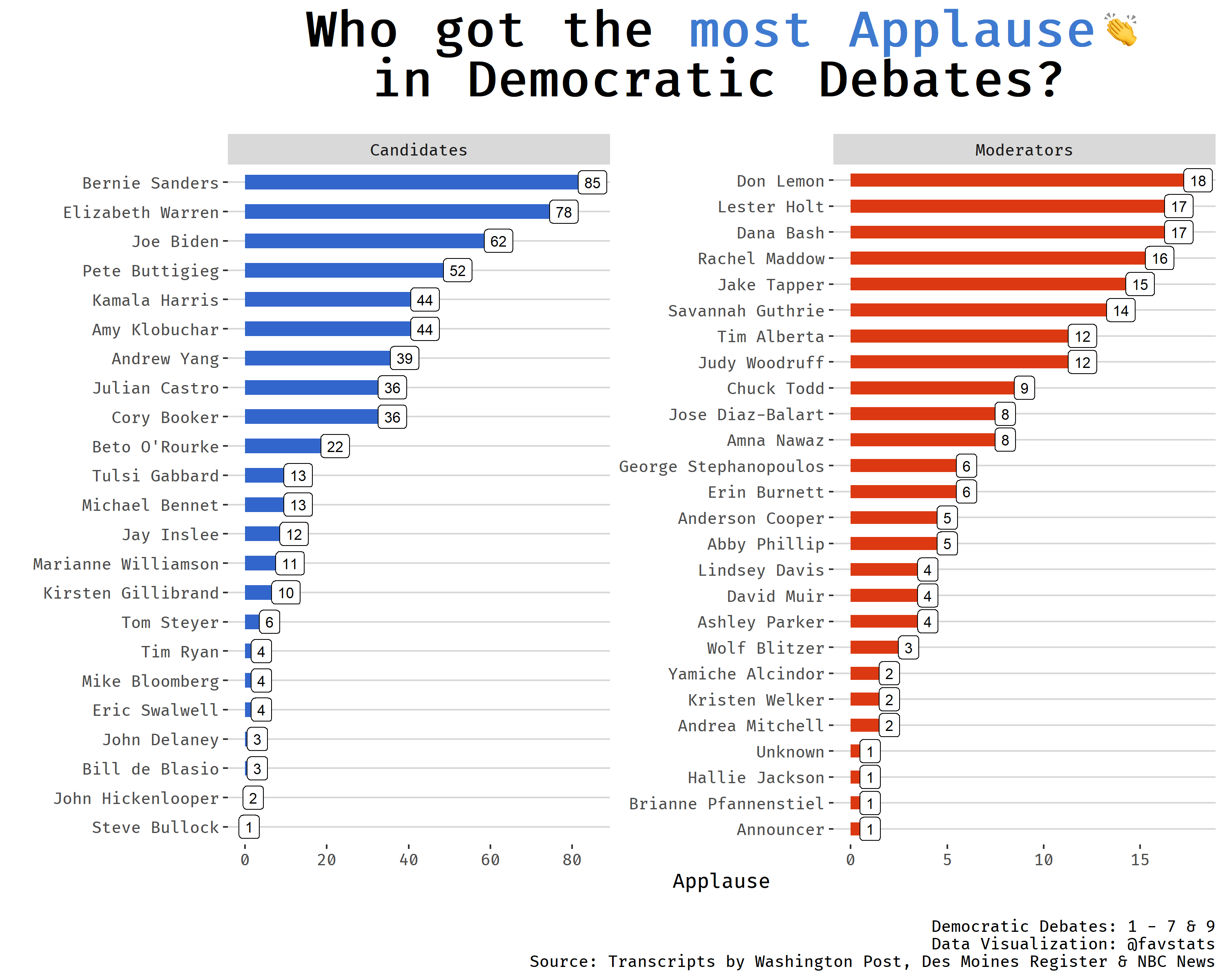
Who received the most applause?
We can use the background variable to see who received the most
applause.
## check out who received Applause
debates %>%
  filter(background == "(APPLAUSE)") %>%
  dplyr::count(speaker, sort = T) %>%
  slice(1:10) %>%
  knitr::kable()
| speaker | n |
|---|---|
| Bernie Sanders | 73 |
| Elizabeth Warren | 65 |
| Joe Biden | 48 |
| Pete Buttigieg | 47 |
| Kamala Harris | 44 |
| Andrew Yang | 39 |
| Cory Booker | 36 |
| Julian Castro | 36 |
| Amy Klobuchar | 32 |
| Beto O’Rourke | 22 |
Looks like Bernie Sanders received the most applause.
We can also create a data visualization to better emphasize the differences.
As mentioned before I will use emojis in the graphs to liven things up. In order to so, I use two functions from the great blogpost Real emojis in ggplot2 by Emil Hvitfeldt.
emoji_to_link <- function(x) {
  paste0("https://emojipedia.org/emoji/",x) %>%
    read_html() %>%
    html_nodes("tr td a") %>%
    .[1] %>%
    html_attr("href") %>%
    paste0("https://emojipedia.org/", .) %>%
    read_html() %>%
    html_node('div[class="vendor-image"] img') %>%
    html_attr("src")
}

link_to_img <- function(x, size = 20) {
  paste0("<img src='", x, "' width='", size, "'/>")
}
Next, I get the emoji link for 👏
clap_emoji <- emoji_to_link("👏") %>% link_to_img()

clap_emoji
## [1] "<img src='https://emojipedia-us.s3.dualstack.us-west-1.amazonaws.com/thumbs/120/apple/237/clapping-hands-sign_1f44f.png' width='20'/>"
And I can include that in a graph:
## load fonts
loadfonts(device = "win")

debates %>%
  dplyr::count(background, speaker, type, sort = T) %>%
  drop_na() %>%
  filter(background == "(APPLAUSE)") %>%
  mutate(speaker = fct_reorder(speaker, n)) %>%
  mutate(type = paste0(type, "s")) %>%
  ggplot(aes(speaker, n)) +
  geom_col(aes(fill = type), width = 0.5) +
  coord_flip() +
  ggthemes::theme_hc() +
  geom_label(aes(label = n), size = 3) +
  facet_wrap(~type, scales = "free") +
  ggthemes::scale_fill_gdocs() +
  theme(
    text = element_text(family = "Fira Code Retina"),
    legend.position = "none",
    plot.title = element_markdown(hjust = 0.5, size = 30, margin=margin(0,0,15,0), face = "bold")
    ) +
  labs(x = "", y = "Applause", title = "Who got the <span style='color: #3E7ACF'>most Applause</span><img src='https://emojipedia-us.s3.dualstack.us-west-1.amazonaws.com/thumbs/120/apple/237/clapping-hands-sign_1f44f.png' width='20'/><br>in Democratic Debates?",
       caption = "\nDemocratic Debates: 1 - 7\nData Visualization: @favstats\nSource: Transcripts by Washington Post & Des Moines Register")
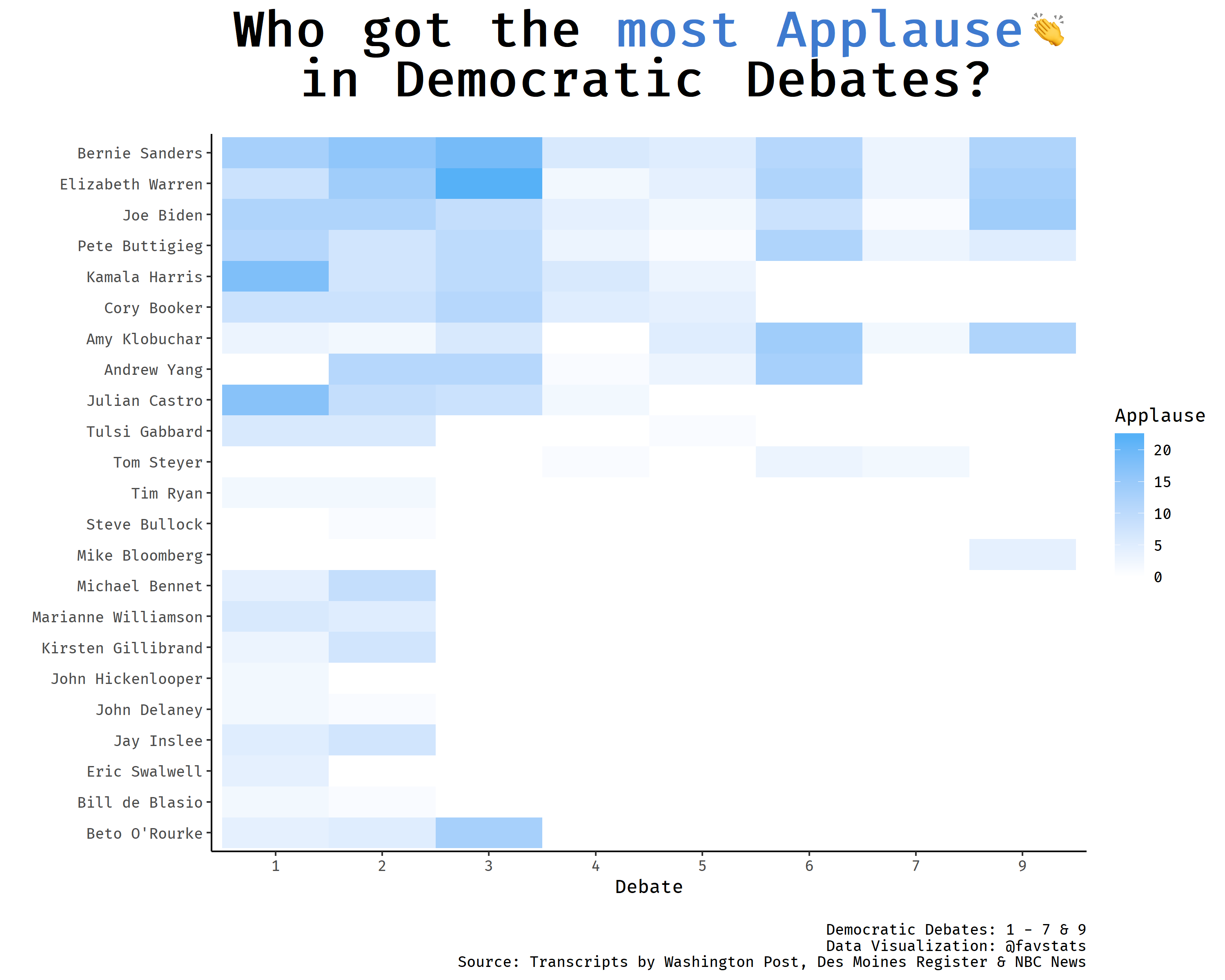
We can also plot the same data as a heatmap across debates:
debates %>%
  filter(background == "(APPLAUSE)") %>%
  filter(type == "Candidate") %>%
  mutate(speaker = as.factor(speaker)) %>%
  mutate(debate = as.factor(debate)) %>%
  dplyr::count(background, speaker, debate, .drop = F) %>%
  drop_na() %>%
  mutate(speaker = fct_reorder(speaker, n)) %>%
  ggplot(aes(debate, speaker, fill = n)) +
  geom_tile() +
  scale_fill_gradient("Applause", low = "white") +
  theme_classic() +
  theme(
    text = element_text(family = "Fira Code Retina"),
    plot.title = element_markdown(hjust = 0.5, size = 30, margin=margin(0,0,15,0), face = "bold")
    ) +
  labs(x = "Debate", y = "", title = "Who got the <span style='color: #3E7ACF'>most Applause</span><img src='https://emojipedia-us.s3.dualstack.us-west-1.amazonaws.com/thumbs/120/apple/237/clapping-hands-sign_1f44f.png' width='20'/><br>in Democratic Debates?",
       caption = "\nDemocratic Debates: 1 - 7\nData Visualization: @favstats\nSource: Transcripts by Washington Post & Des Moines Register")
Who was the greatest jokester at democratic debates?
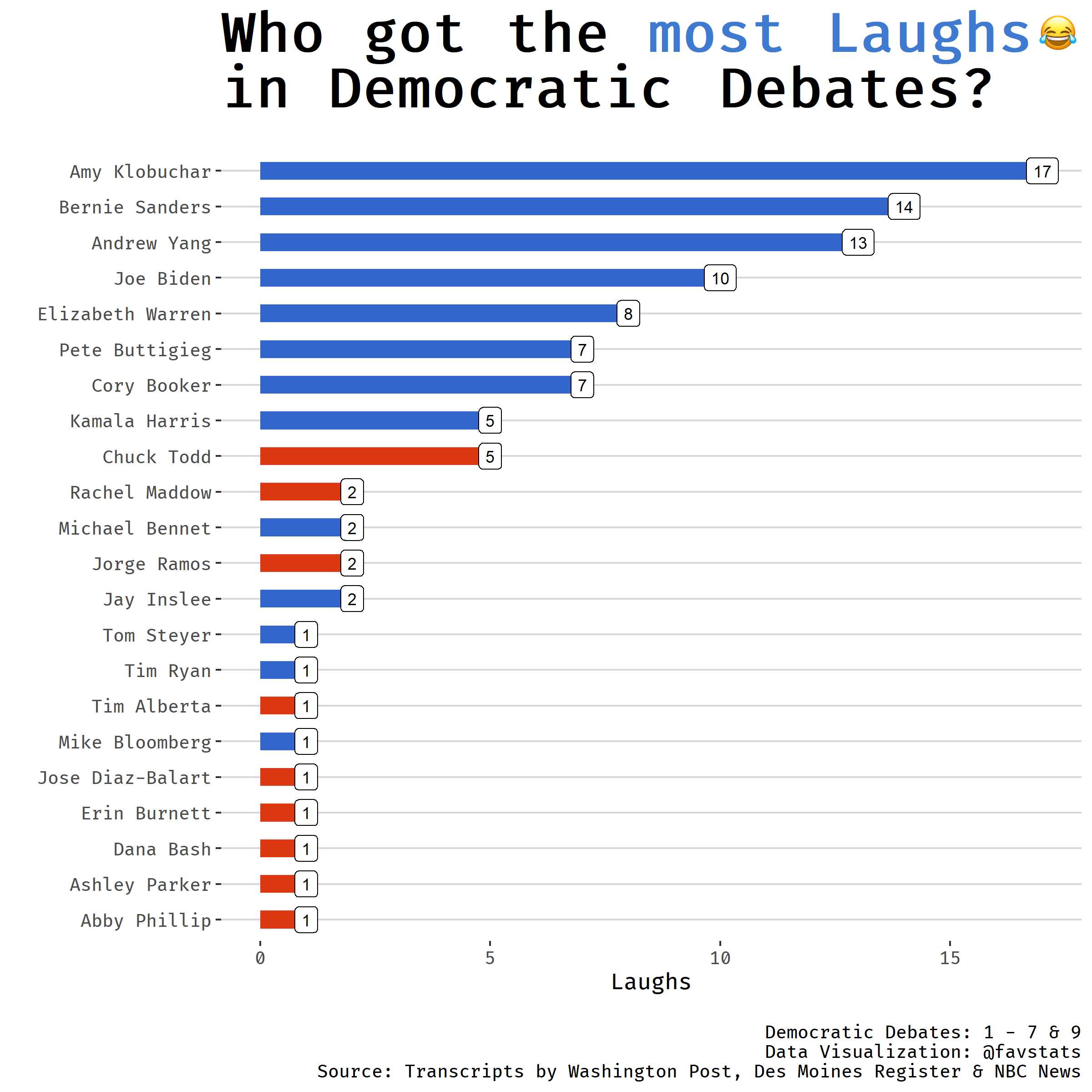
We can also take a look at who received the most laughs during the
debates. Just filter background by (LAUGHTER).
debates %>%
  filter(background == "(LAUGHTER)") %>%
  dplyr::count(speaker, sort = T) %>%
  drop_na() %>%
  slice(1:10) %>%
  knitr::kable()
| speaker | n |
|---|---|
| Bernie Sanders | 14 |
| Amy Klobuchar | 13 |
| Andrew Yang | 13 |
| Joe Biden | 9 |
| Elizabeth Warren | 8 |
| Cory Booker | 7 |
| Pete Buttigieg | 6 |
| Kamala Harris | 5 |
| Chuck Todd | 3 |
| Jay Inslee | 2 |
Again, Bernie Sanders leads the field, closely followed by Andrew Yang (now dropped out) and Amy Klobuchar.
We can visualize the data to get a better understanding. With the same process as before, I get the emoji link for 😂
laugh_emoji <- emoji_to_link("😂") %>% link_to_img()

laugh_emoji
## [1] "<img src='https://emojipedia-us.s3.dualstack.us-west-1.amazonaws.com/thumbs/120/apple/237/face-with-tears-of-joy_1f602.png' width='20'/>"
And I can include that in a graph:
debates %>%
  filter(background == "(LAUGHTER)") %>%
  dplyr::count(background, speaker, type, sort = T) %>%
  drop_na() %>%
  mutate(speaker = fct_reorder(speaker, n)) %>%
  ggplot(aes(speaker, n)) +
  geom_col(aes(fill = type), width = 0.5) +
  # geom_point(aes(fill = type), size = 9) +
  coord_flip() +
  ggthemes::theme_hc() +
  geom_label(aes(label = n), size = 3) +
  # facet_grid(~type, scales = "free_x", space = "free") +
  ggthemes::scale_fill_gdocs() +
  theme(
    text = element_text(family = "Fira Code Retina"),
    legend.position = "none",
    plot.title = element_markdown(size = 30, margin=margin(0,0,15,0), face = "bold")
    ) +
  labs(x = "", y = "Laughs", title = "Who got the <span style='color: #3E7ACF'>most Laughs</span><img src='https://emojipedia-us.s3.dualstack.us-west-1.amazonaws.com/thumbs/120/apple/237/face-with-tears-of-joy_1f602.png' width='20'/><br>in Democratic Debates?",
       caption = "\nDemocratic Debates: 1 - 7\nData Visualization: @favstats\nSource: Transcripts by Washington Post & Des Moines Register")
tidytemplate::ggsave_it(laughs, width = 8, height = 8)
We can also plot the same data as a heatmap across debates:
debates %>%
  filter(background == "(LAUGHTER)") %>%
  filter(type == "Candidate") %>%
  mutate(speaker = as.factor(speaker)) %>%
  mutate(debate = as.factor(debate)) %>%
  dplyr::count(background, speaker, debate, .drop = F) %>%
  drop_na() %>%
  mutate(speaker = fct_reorder(speaker, n)) %>%
  ggplot(aes(debate, speaker, fill = n)) +
  geom_tile() +
  scale_fill_gradient("Laughs", low = "white") +
  theme_classic() +
  theme(
    text = element_text(family = "Fira Code Retina"),
    plot.title = element_markdown(hjust = 0.5, size = 30, margin=margin(0,0,15,0), face = "bold")
    ) +
  labs(x = "Debate", y = "", title = "Who got the <span style='color: #3E7ACF'>most Laughs</span><img src='https://emojipedia-us.s3.dualstack.us-west-1.amazonaws.com/thumbs/120/apple/237/face-with-tears-of-joy_1f602.png' width='20'/><br>in Democratic Debates?",
       caption = "\nDemocratic Debates: 1 - 7\nData Visualization: @favstats\nSource: Transcripts by Washington Post & Des Moines Register")

Who spoke the most words?
debates %>%
  unnest_tokens(word, speech) %>%
  filter(type == "Candidate") %>%
  mutate(speaker = as.factor(speaker)) %>%
  mutate(debate = as.factor(debate)) %>%
  dplyr::count(speaker, .drop = F, sort = T) %>%
  mutate(total = sum(n)) %>%
  mutate(perc = round(n / total*100, 2)) %>%
  slice(1:10) %>%
  knitr::kable()
| speaker | n | total | perc |
|---|---|---|---|
| Joe Biden | 25295 | 201653 | 12.54 |
| Elizabeth Warren | 22473 | 201653 | 11.14 |
| Pete Buttigieg | 21400 | 201653 | 10.61 |
| Amy Klobuchar | 20076 | 201653 | 9.96 |
| Bernie Sanders | 19065 | 201653 | 9.45 |
| Kamala Harris | 12128 | 201653 | 6.01 |
| Cory Booker | 11839 | 201653 | 5.87 |
| Andrew Yang | 10586 | 201653 | 5.25 |
| Tom Steyer | 9635 | 201653 | 4.78 |
| Beto O’Rourke | 8253 | 201653 | 4.09 |
In the Top 10 we see candidates who were present in each debate (for example Joe Biden, Elizabeth Warren and Bernie Sanders). Out of a share of all spoken words during all eight debates, Joe Biden spoke a plurality of words. Tom Steyer (as of writing still in the race) has less than half as many spoken words as most other candidates still in the race, despite being present in 5 out of 8 debates.
Again, we can also visualize the data.
speak_emoji <- emoji_to_link("🗣") %>% link_to_img()

speak_emoji
## [1] "<img src='https://emojipedia-us.s3.dualstack.us-west-1.amazonaws.com/thumbs/120/apple/237/speaking-head-in-silhouette_1f5e3.png' width='20'/>"
debate_words <- debates %>%
  unnest_tokens(word, speech) %>%
  filter(type == "Candidate") %>%
  mutate(speaker = as.factor(speaker)) %>%
  mutate(debate = as.factor(debate)) %>%
  dplyr::count(speaker, debate, .drop = F, sort = T)

# frontrunners <- c("Bernie Sanders",
#                   "Elizabeth Warren",
#                   "Joe Biden",
#                   "Pete Buttigieg",
#                   "Amy Klobuchar")


debate_words %>%
  mutate(speaker = fct_reorder(speaker, n)) %>%
  ggplot(aes(debate, speaker, fill = n)) +
  geom_tile() +
  scale_fill_gradient("Words", low = "white") +
  theme_classic() +
  theme(
    text = element_text(family = "Fira Code Retina"),
    plot.title = element_markdown(hjust = 0.5, size = 30, margin=margin(0,0,15,0), face = "bold")
    ) +
  labs(x = "Debate", y = "", title = "Who spoke the <span style='color: #3E7ACF'>most Words</span><img src='https://emojipedia-us.s3.dualstack.us-west-1.amazonaws.com/thumbs/120/apple/237/speaking-head-in-silhouette_1f5e3.png' width='20'/><br>in Democratic Debates?",
       caption = "\nDemocratic Debates: 1 - 8\nData Visualization: @favstats\nSource: Transcripts by Washington Post & Des Moines Register")
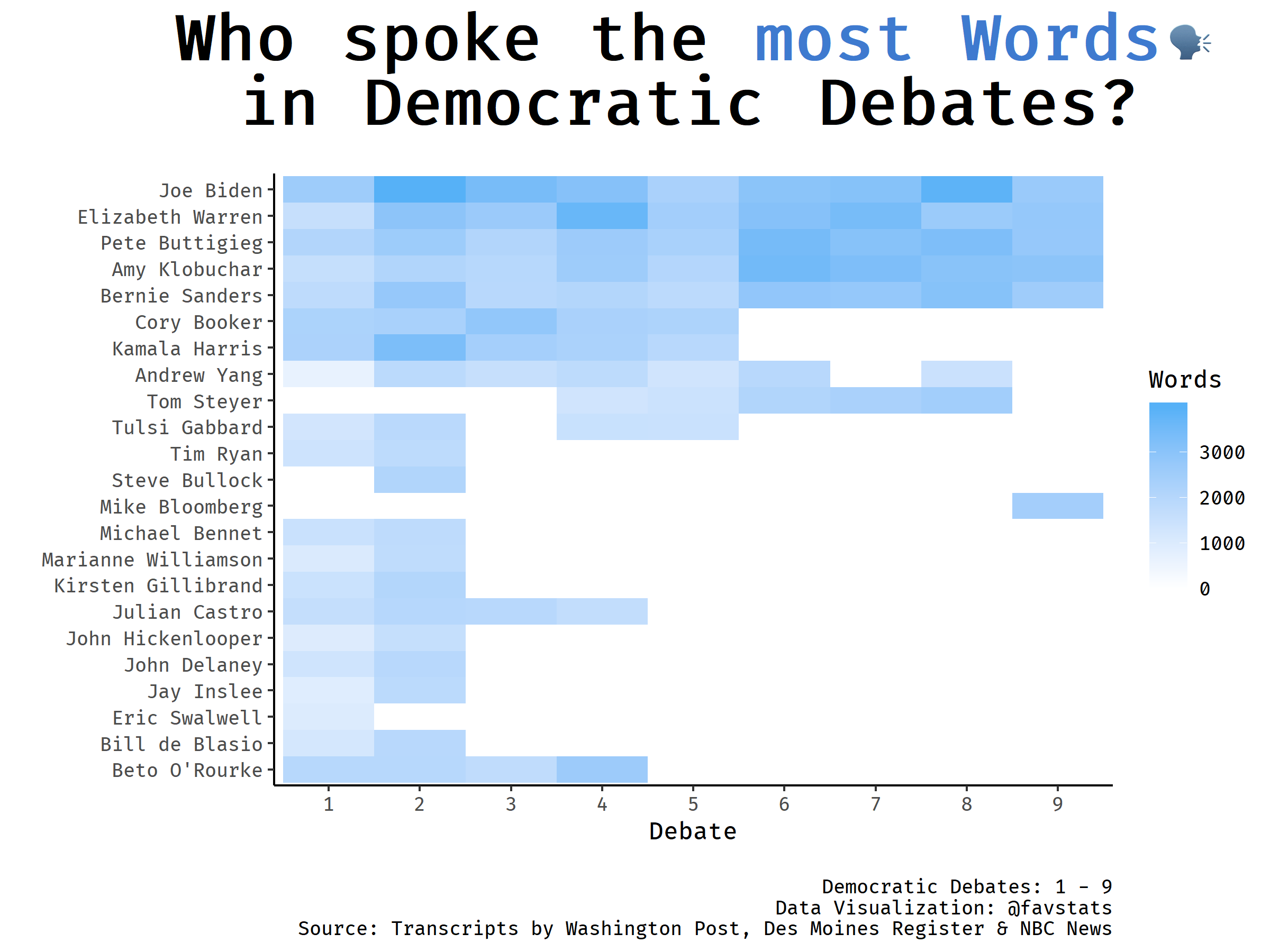
We see something very obvious: as the number of candidates decreases, the spoken words also increase for the remaining candidates (as they have to fill the space). Numbers remain rather low for Tom Steyer and Andrew Yang throughout the debates.
Did men speak more than women?
debate_gender <- debates %>%
  unnest_tokens(word, speech) %>%
  filter(type == "Candidate") %>%
  dplyr::count(gender, debate, .drop = F) %>%
  group_by(debate) %>%
  mutate(total = sum(n)) %>%
  mutate(perc = n/total)

debate_gender %>%
  filter(gender == "female") %>%
  ggplot(aes(debate, perc, fill = gender)) +
  geom_area(fill = "#3E7ACF", alpha = 0.75) +
  ggrepel::geom_text_repel(aes(label = paste0(round(perc*100, 1), "%")), nudge_y = 0.025,
                           direction = "y") +
  scale_y_continuous(labels = scales::percent, limits = c(0, 0.5)) +
  ggthemes::theme_hc()  +
  theme(
    text = element_text(family = "Fira Code Retina"),
    legend.position = "top",
    plot.title = element_markdown(size = 25, margin=margin(0,0,15,0), face = "bold")
    ) +
  labs(x = "", y = "% Spoken Words by Women\n", title = "Share of spoken Words by <span style='color: #3E7ACF'>Women</span><br>during the Democratic Debates",
       caption = "\nDemocratic Debates: 1 - 8\nData Visualization: @favstats\nSource: Transcripts by Washington Post & Des Moines Register") +
  scale_x_continuous(breaks = 1:8)
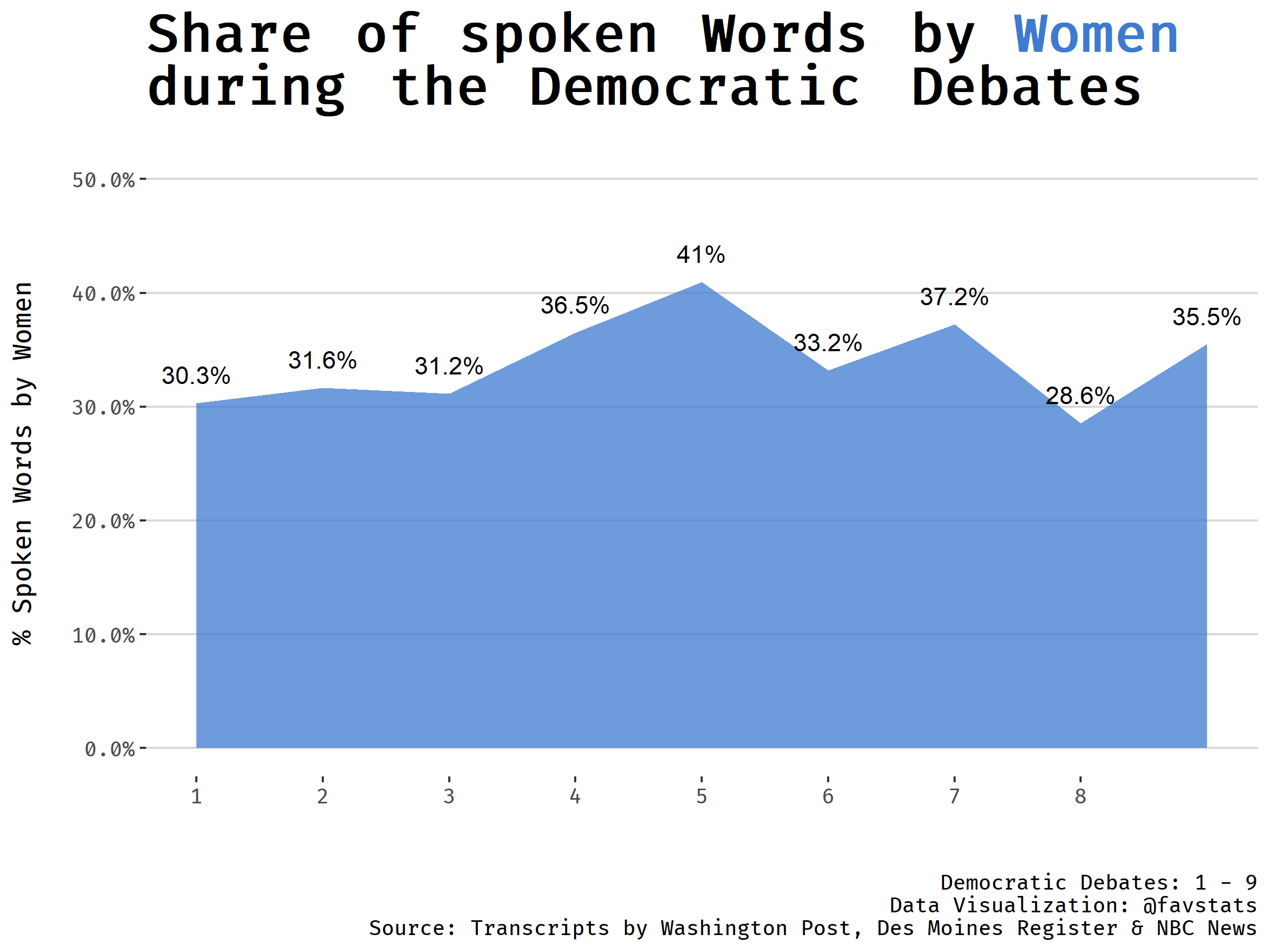
Men have spoken more words than women across all debates. Of course, throughout the debates women were always in the minority (only 6 out of 22 Democratic candidates were women and now only 2 are left: Amy Klobuchar and Elizabeth Warren).
What were the most common distinct words used by candidates?
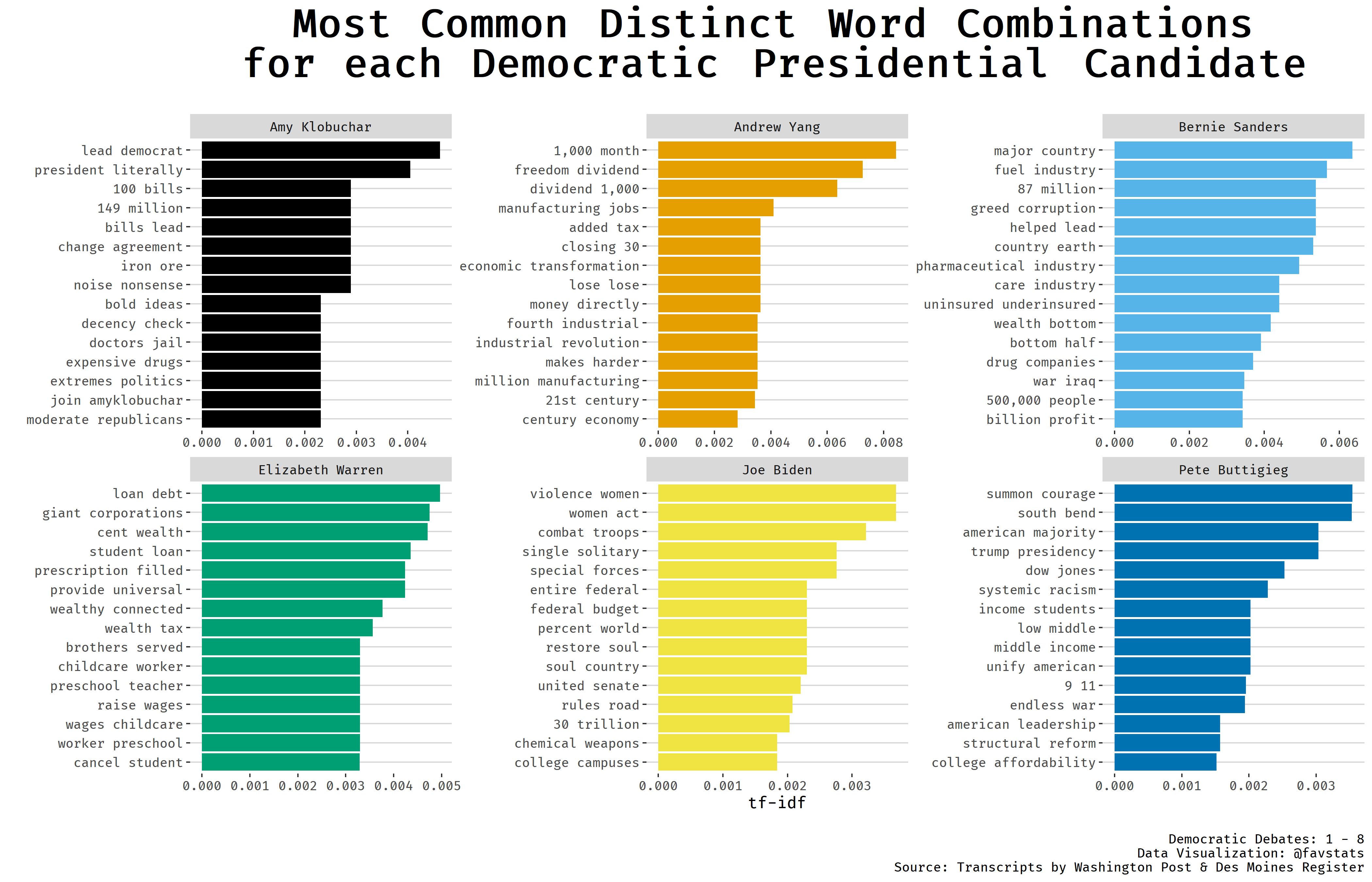
We can use tf-idf scores to tell what word combinations (bigrams) candidates used the most and also were most distinct across other candidates.
speaker_words <- debates %>%
  filter(type == "Candidate") %>%
  mutate(speech = tm::removeWords(str_to_lower(speech), stop_words$word)) %>%
  unnest_tokens(word, speech, token = "ngrams", n = 2) %>%
  count(speaker, word, sort = TRUE)

total_words <- speaker_words %>%
  group_by(speaker) %>%
  summarize(total = sum(n))


speaker_words <- left_join(speaker_words, total_words)


speaker_words <- speaker_words %>%
  bind_tf_idf(word, speaker, n)


speaker_words %>%
  arrange(desc(tf_idf)) %>%
  filter(speaker %in% c("Bernie Sanders", "Elizabeth Warren",
                        "Joe Biden", "Pete Buttigieg",
                        "Andrew Yang", "Amy Klobuchar")) %>%
  group_by(speaker) %>%
  arrange(desc(tf_idf)) %>%
  slice(1:15) %>%
  ungroup() %>%
  mutate(word = factor(word, levels = rev(unique(word)))) %>%
  ggplot(aes(word, tf_idf, fill = speaker)) +
  geom_col(show.legend = FALSE) +
  labs(x = NULL, y = "tf-idf") +
  facet_wrap(~speaker, ncol = 3, scales = "free") +
  coord_flip()   +
  ggthemes::theme_hc() +
  # facet_grid(~type, scales = "free_x", space = "free") +
  ggthemes::scale_fill_colorblind() +
  theme(
    text = element_text(family = "Fira Code Retina"),
    legend.position = "top",
    plot.title = element_markdown(size = 30, margin=margin(0,0,20,0), face = "bold", hjust = 0.5)
    ) +
  labs(x = "", y = "tf-idf", title = "Most Common Distinct Word Combinations<br>for each Democratic Presidential Candidate",
       caption = "\nDemocratic Debates: 1 - 8\nData Visualization: @favstats\nSource: Transcripts by Washington Post & Des Moines Register")
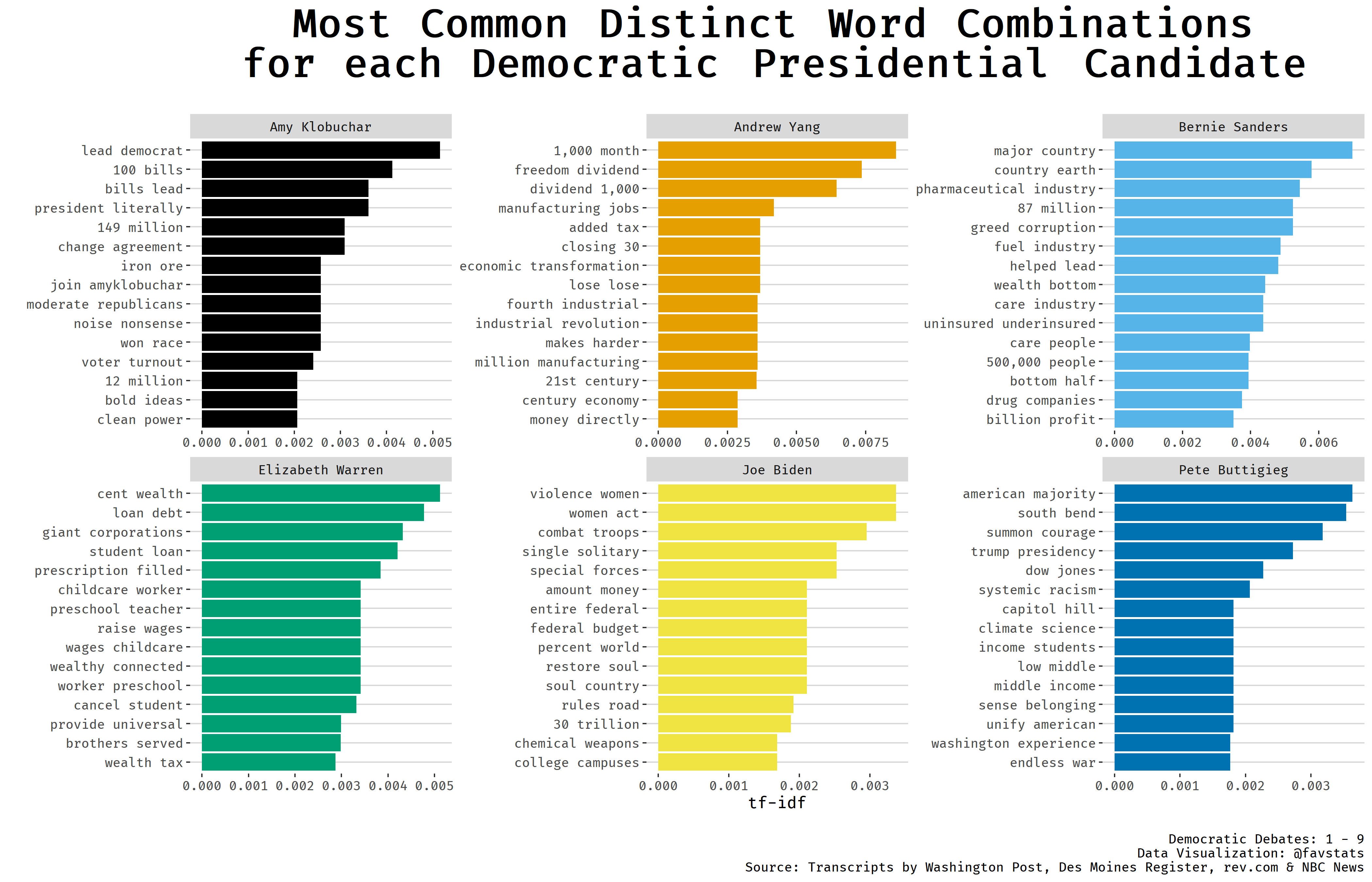
Some fitting and recognizable word patterns emerge. For exampe, Andrew Yang and his proposal for Universal Basic Income (UBI) clearly distinguish him from other candidates with his most common distinct words referring to the “freedom dividend” and “1000 [dollars a] month”. A similar distinct pattern emerges with Bernie Sanders who frequently uses the phrase “The US is the only major country on earth that does/does not have X”.
In conclusio
So far from me. What kind of analysis would you run on the Democratic debates data? Feel free to use the data as you wish and I am curious to see what comes out of it!
sessionInfo()
## R version 3.6.1 (2019-07-05)
## Platform: x86_64-w64-mingw32/x64 (64-bit)
## Running under: Windows 10 x64 (build 18362)
##
## Matrix products: default
##
## locale:
## [1] LC_COLLATE=English_Germany.1252  LC_CTYPE=English_Germany.1252
## [3] LC_MONETARY=English_Germany.1252 LC_NUMERIC=C
## [5] LC_TIME=English_Germany.1252
##
## attached base packages:
## [1] stats     graphics  grDevices utils     datasets  methods   base
##
## other attached packages:
##  [1] scales_1.1.0              ggthemes_4.2.0
##  [3] demdebates2020_0.0.0.9000 tidytext_0.2.2
##  [5] rvest_0.3.4               xml2_1.2.2
##  [7] ggtext_0.1.0              extrafont_0.17
##  [9] knitr_1.25                forcats_0.4.0
## [11] stringr_1.4.0             dplyr_0.8.3
## [13] purrr_0.3.3               readr_1.3.1
## [15] tidyr_1.0.0               tibble_2.1.3
## [17] ggplot2_3.2.1             tidyverse_1.2.1
##
## loaded via a namespace (and not attached):
##  [1] httr_1.4.1         jsonlite_1.6       modelr_0.1.5
##  [4] assertthat_0.2.1   highr_0.8          tidytemplate_0.1.0
##  [7] selectr_0.4-1      cellranger_1.1.0   slam_0.1-45
## [10] yaml_2.2.0         ggrepel_0.8.1      Rttf2pt1_1.3.7
## [13] pillar_1.4.3       backports_1.1.5    lattice_0.20-38
## [16] glue_1.3.1         extrafontdb_1.0    digest_0.6.23
## [19] gridtext_0.1.0     colorspace_1.4-1   htmltools_0.4.0
## [22] Matrix_1.2-17      tm_0.7-7           pkgconfig_2.0.3
## [25] broom_0.5.2        haven_2.1.1        generics_0.0.2
## [28] farver_2.0.1       ellipsis_0.3.0     pacman_0.5.1
## [31] withr_2.1.2        lazyeval_0.2.2     NLP_0.2-0
## [34] cli_2.0.0          magrittr_1.5       crayon_1.3.4
## [37] readxl_1.3.1       evaluate_0.14      tokenizers_0.2.1
## [40] janeaustenr_0.1.5  fansi_0.4.0        nlme_3.1-140
## [43] SnowballC_0.6.0    tools_3.6.1        hms_0.5.2
## [46] lifecycle_0.1.0    munsell_0.5.0      compiler_3.6.1
## [49] rlang_0.4.1        grid_3.6.1         RCurl_1.95-4.12
## [52] rstudioapi_0.10    bitops_1.0-6       labeling_0.3
## [55] rmarkdown_1.14     gtable_0.3.0       curl_4.2
## [58] markdown_1.1       R6_2.4.1           lubridate_1.7.4
## [61] zeallot_0.1.0      stringi_1.4.3      parallel_3.6.1
## [64] Rcpp_1.0.3         vctrs_0.2.1        png_0.1-7
## [67] tidyselect_0.2.5   xfun_0.10
